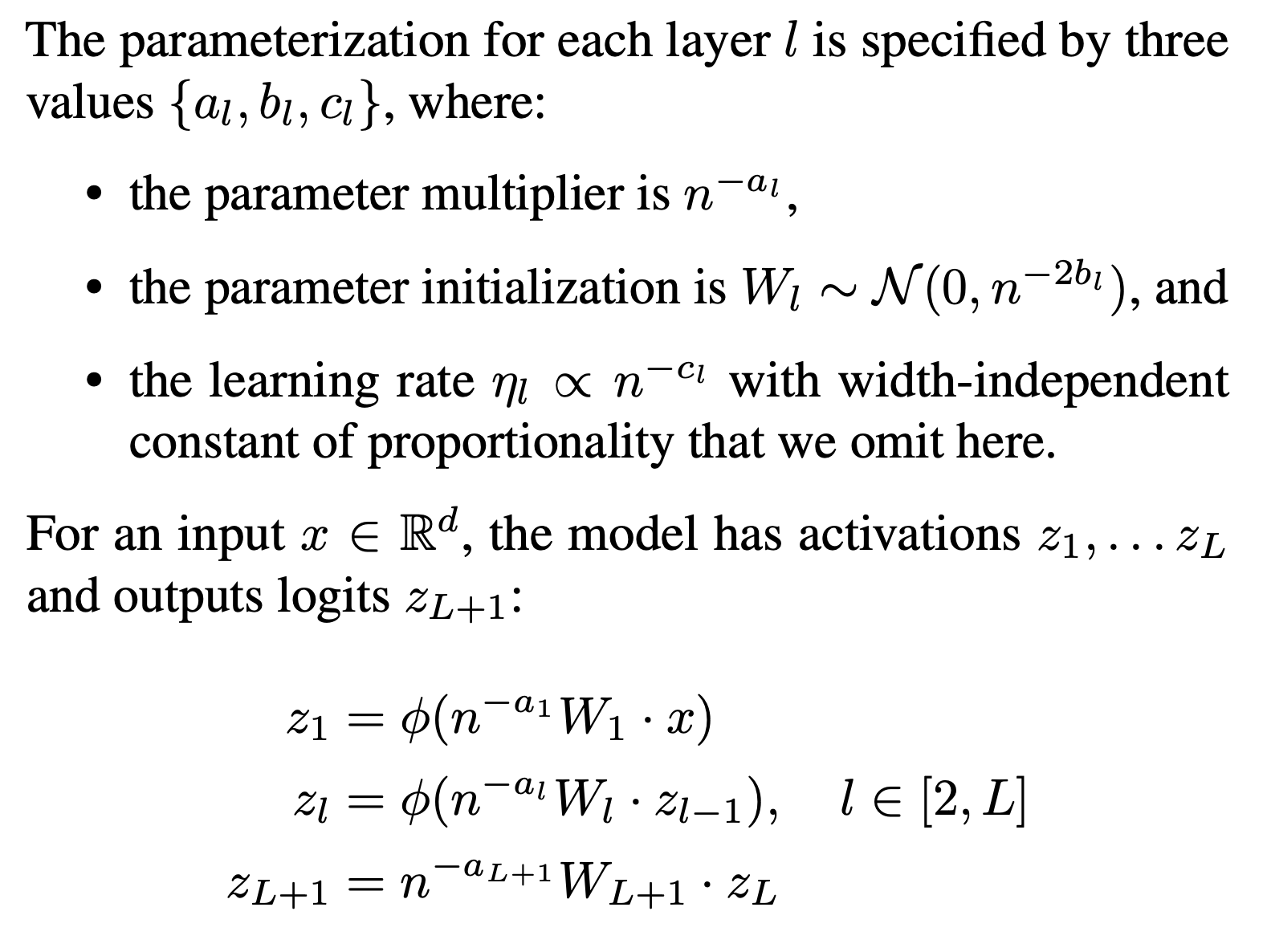
Exploring Tensor Alignments in Neural Networks
This document summarizes our exploration into neural network parameterizations, focusing specifically on the abc-parameterization framework defined in [1], with width serving as our primary scaling axis.
In the end we develop a dynamic learning rate scheduler which solves for the maximal stable learning rate at each step of training by measuring alignments between weights and activations. Using this scheduler we are able to minimize loss more effectively in the majority of cases.
Parameterizations
Let’s examine a simple example for how to design a parameterization to combat instabilities - a single linear weight matrix acting on an input vector.
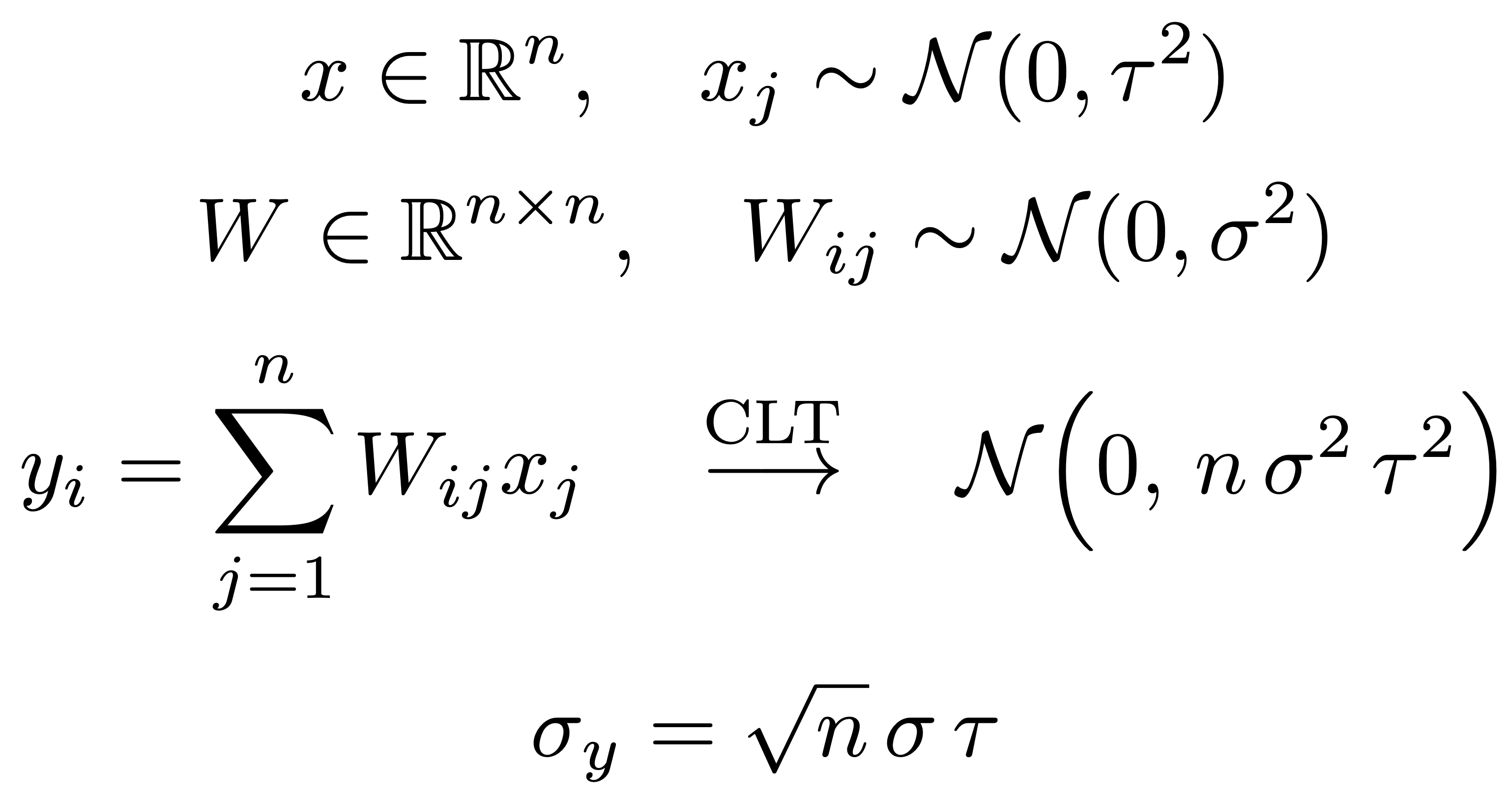
If we naively parametrize our weight matrix, the average coordinate scale is O(sqrt(n)) - this isn’t great if we want to scale model width on hardware with finite precision. Let’s fix this with a parameter multiplier:
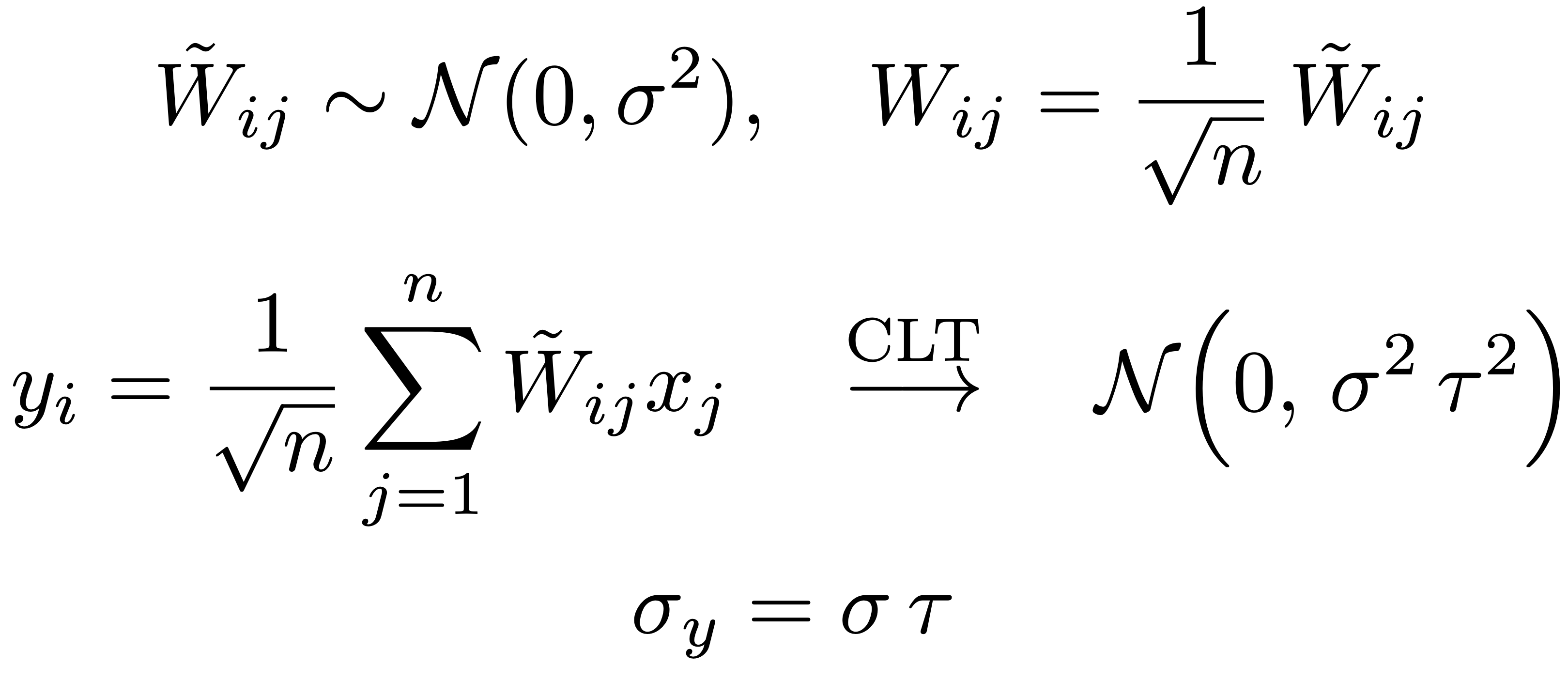
With the 1/sqrt(n) multiplier, for any width we decide to go with, our matrix-vector product will be stable since the coordinate scale is no longer a function of the width.
One limitation of this example is its idealistic assumption that W and x are independently sampled with zero mean, allowing us to apply the Central Limit Theorem. This is only true at initialization when both are randomly drawn from zero-mean distributions. After the first update, we must consider potential alignments between W and x.
Consider an extreme case: if during the first optimizer update, all rows of W were transformed into x.T, the product would scale as O(n) rather than O(sqrt(n)) - they would be fully aligned. Many researchers assume this “full alignment” [5, 6] after training sufficiently warms up and design “defensive” parameterizations to ensure stability under these extreme conditions. However, in [1] they measure the log-alignment ratio and demonstrate this is often overly conservative, suggesting performance gains are possible by relaxing these alignment assumptions.
Solving for Optimal Parametrizations
In numerical optimization we want our algorithms to be fast and stable. These two qualities exist in tension, creating an inevitable tradeoff. Pushing for speed positions work at the stability boundary [2, 3] where small changes in experimental setup can nudge us off the edge. What functions reliably at one scale may fail at another, with instabilities often remaining hidden until deployment at scale.
We can analyze an important aspect of training multi-layer neural networks with the following representative model:
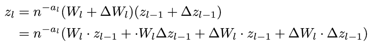
This equation captures how perturbations in weights and activations propagate through the network during training.
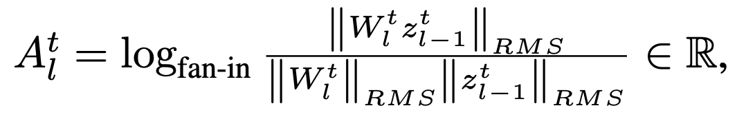
The optimal parameterization maximizes convergence speed while maintaining training stability. To derive such parameterizations, we need clear objectives. The first is straightforward—we want to maximize learning rate. The second requires more nuance. For a comprehensive discussion on this topic, we recommend [1], from which we borrow the following definition:

Intuitively, when r_l = 0, the change in activations remains constant scale regardless of width scaling. Any deviation from this equilibrium pushes us toward either vanishing or exploding activation changes, resulting in poor performance or instability, respectively.
With our neural network training dynamics and stability metric described using math, we can now analyze alignment effects. We can examine the log-alignment ratio for each term in the representative model (except the first term, since we have no alignment during initialization).
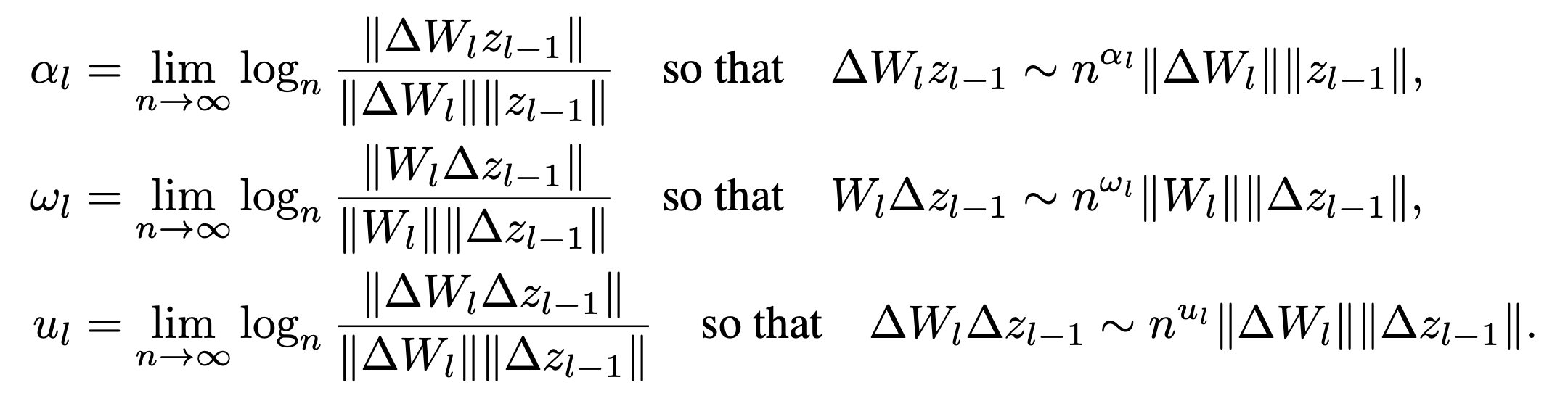
And derive a system of equations and inequalities which describe stable training by ensuring that our stability constraints are met during each training step (see Appendix of [1] for derivation):
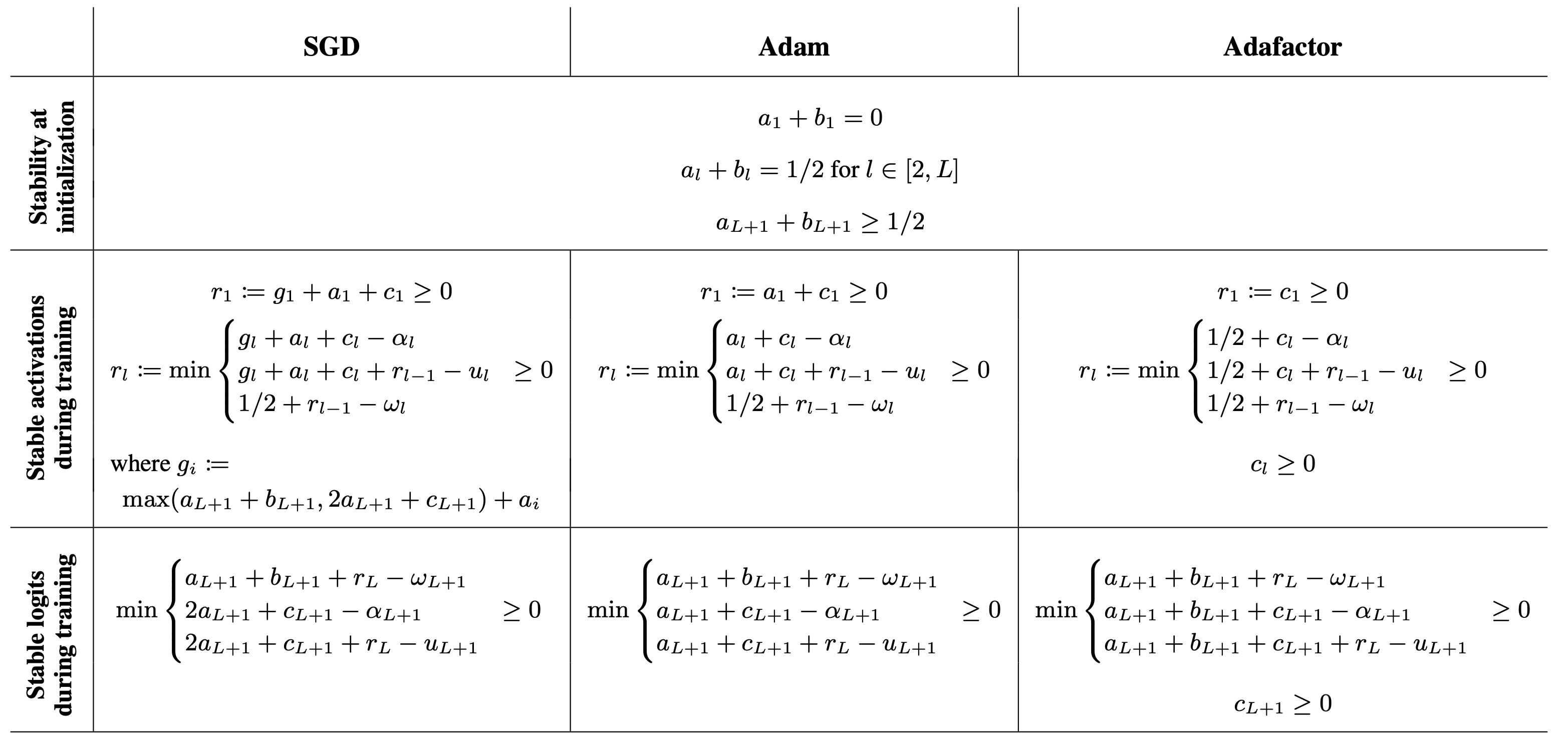
Seeing the Parametrization Landscape
To verify our understanding and theory, we can create a visualization - let’s grab an interesting point on the polyhedron defined by the above system of equations and inequalities, like muP [4], and probe around it. At each point, we can check if the system is satisfied and also train a simple neural network to measure the scale of the change in acitvations.
We can borrow the nice visualization from [2]:
- MLPs with 3 layers and a hidden dimension of 64, using ReLU
- Synthetic data where the input dataset is sampled from an 8-dimensional standard Gaussian and output is sampled from 1-dimensional standard Gaussian
- Training with MSE, full-batch gradient descent for 500 steps of SGD
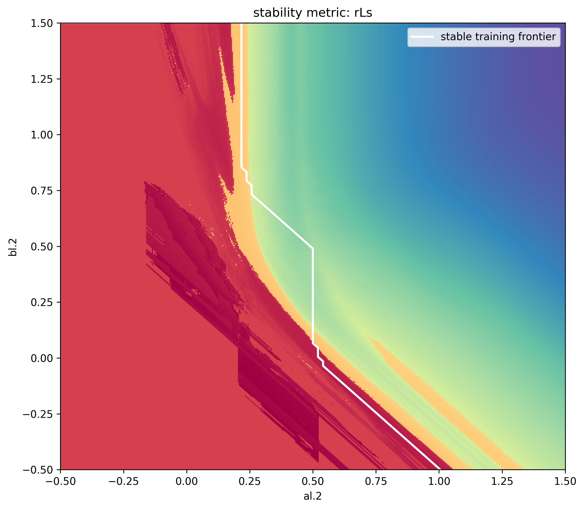
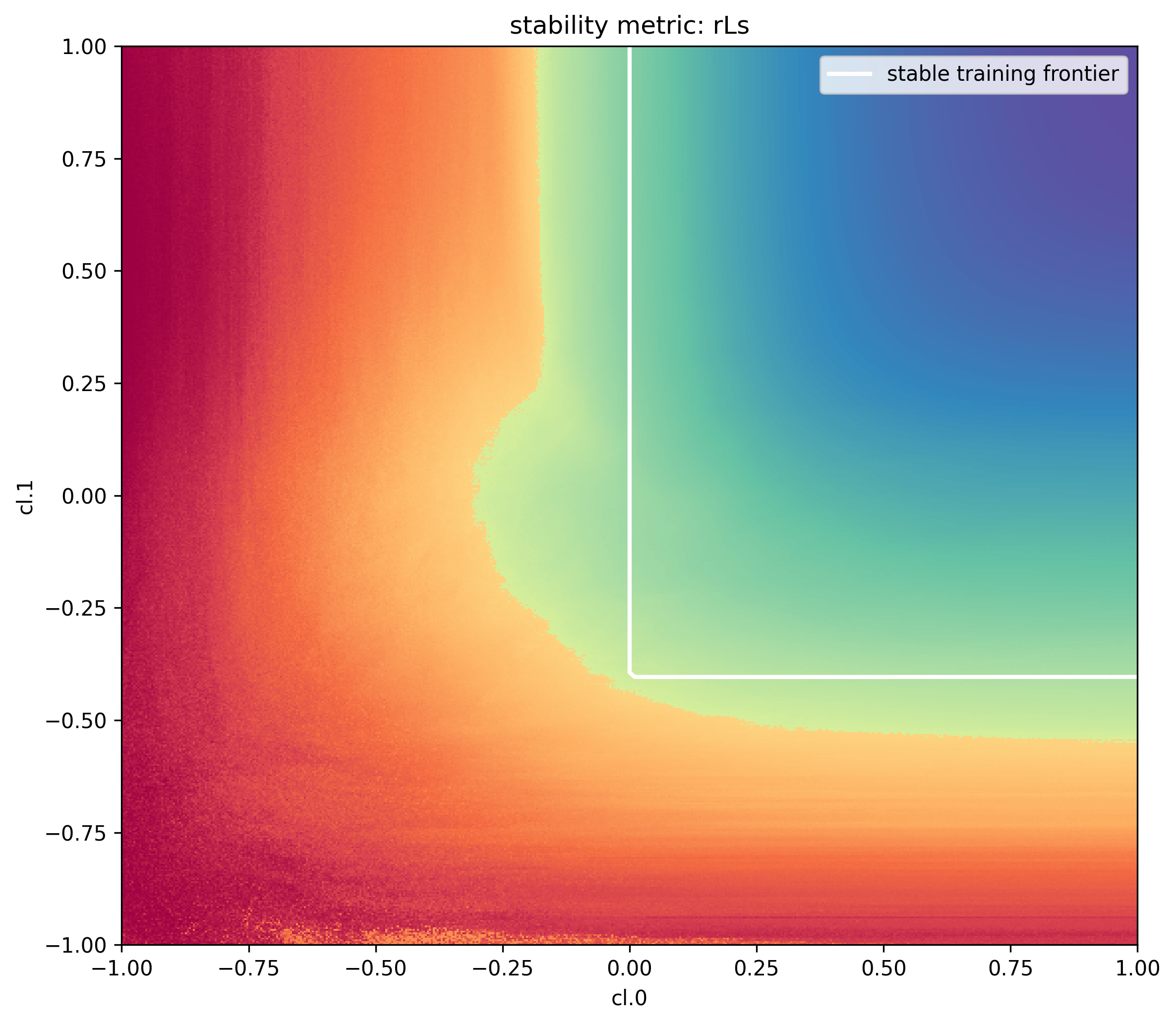
To make 2D plots, let’s explore 2 slices of our parameterization space - a_3 vs b_3 and c_1 vs c_2. These correspond to the last layer parameter multiplier exponent vs. the last layer initialization variance exponent and the first layer learning rate exponent vs. the second layer learning rate exponent. For each, we’ll center the graph at the muP parameterization and assume full alignment.
- The color of each pixel represents the mean scale of change in activations (compared to initialization) in the last 100 steps of training (darker red means more divergence, darker blue means vanishing to 0)
- The best models are trained where this change is constant scale (i.e., 0), which will appear as bright blue colors
- On each graph, we will overlay the boundary of stability (where rL = 0) according to the system of equations and inequalities
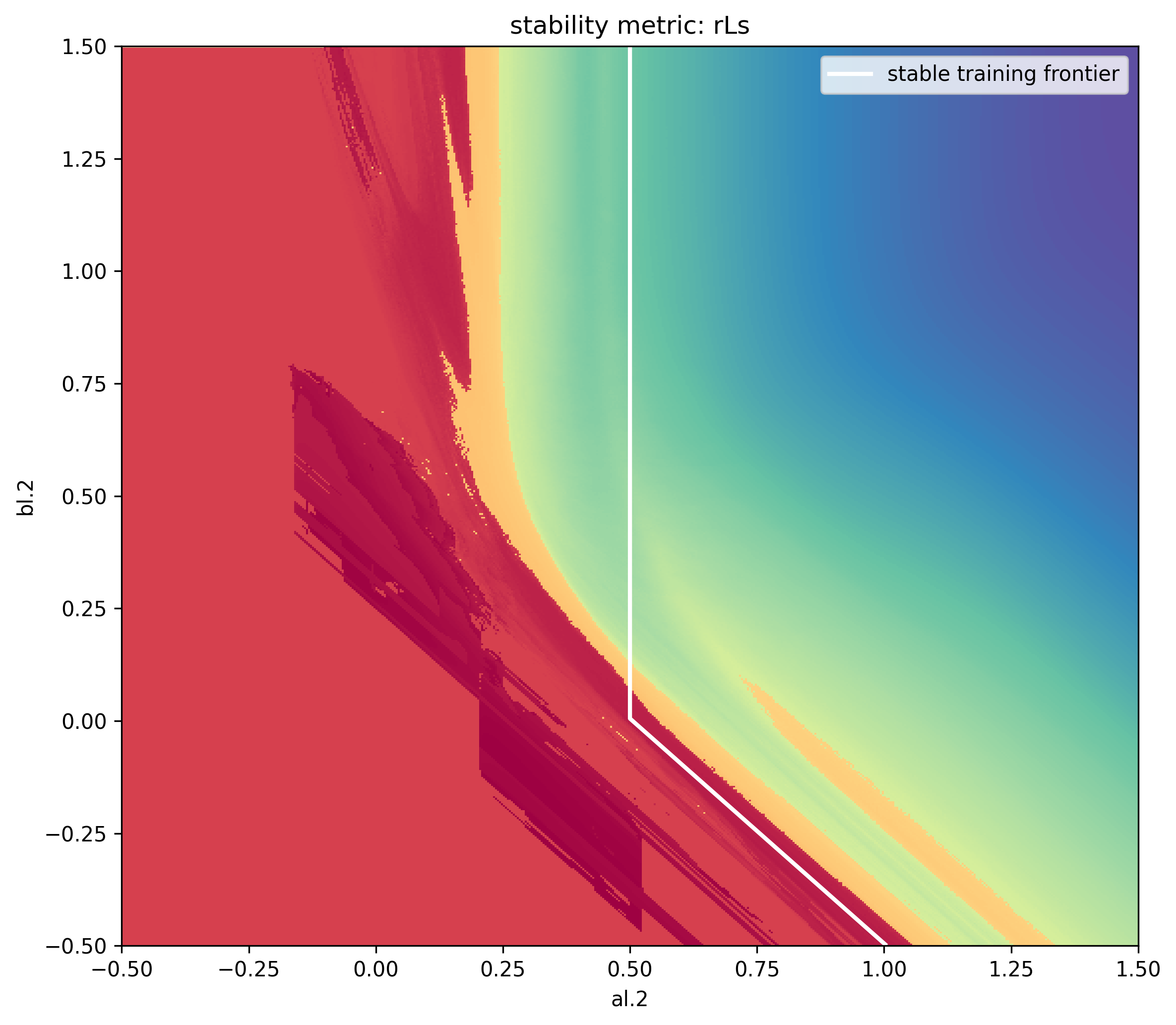
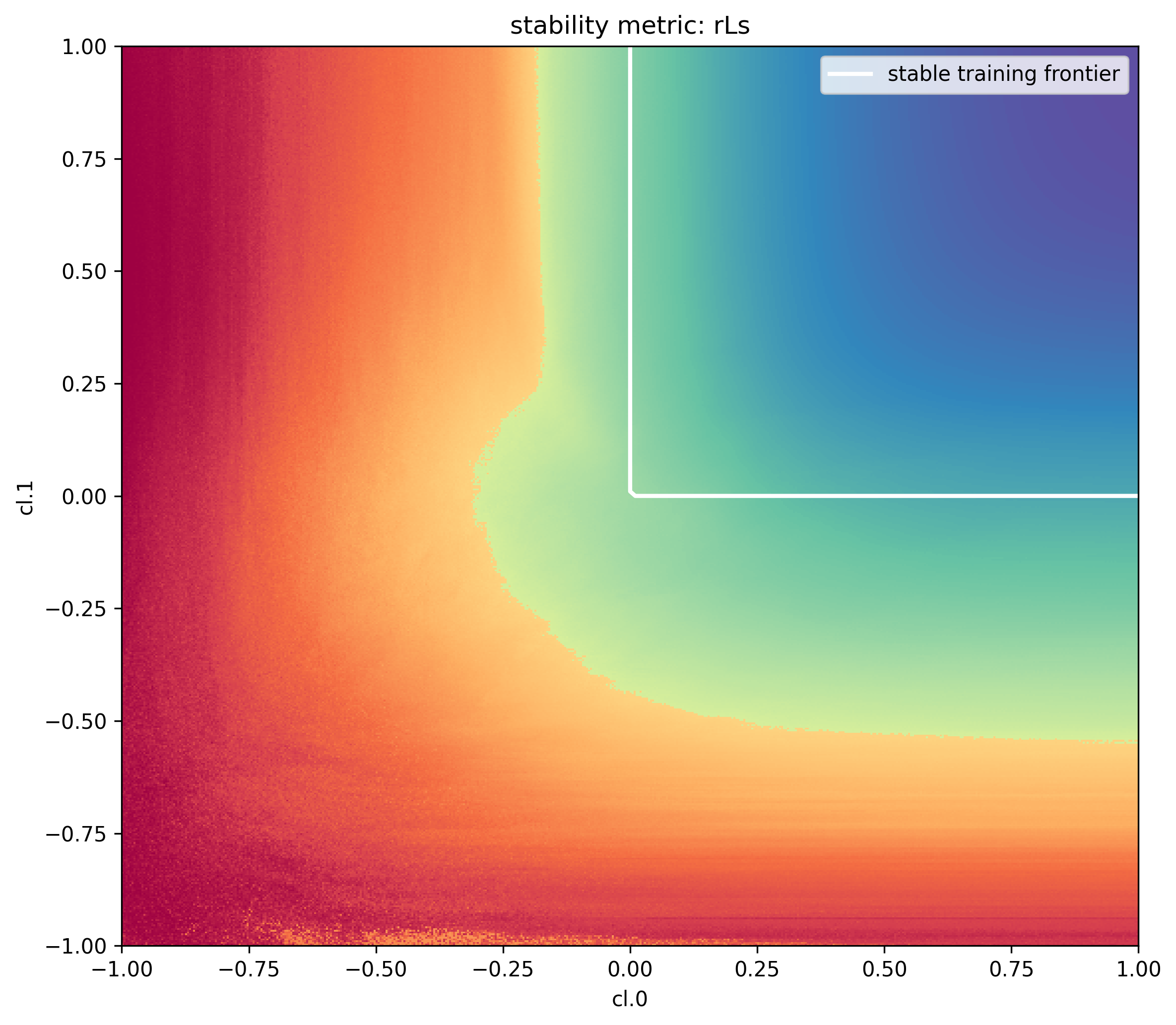
These visualizations show strong overlap with our theoretical predictions and practical results. However, discrepancies appear in two regions: to the left and below the stable training frontier in the left grid, and the right grid respectively. Could our full alignment assumptions be creating overly restrictive constraints? To investigate this hypothesis, let’s examine one experiment from the figure above and track how its alignment variables evolve throughout the training process. For these per-layer metrics we tint the color of the curve darker proportional to the layer index.
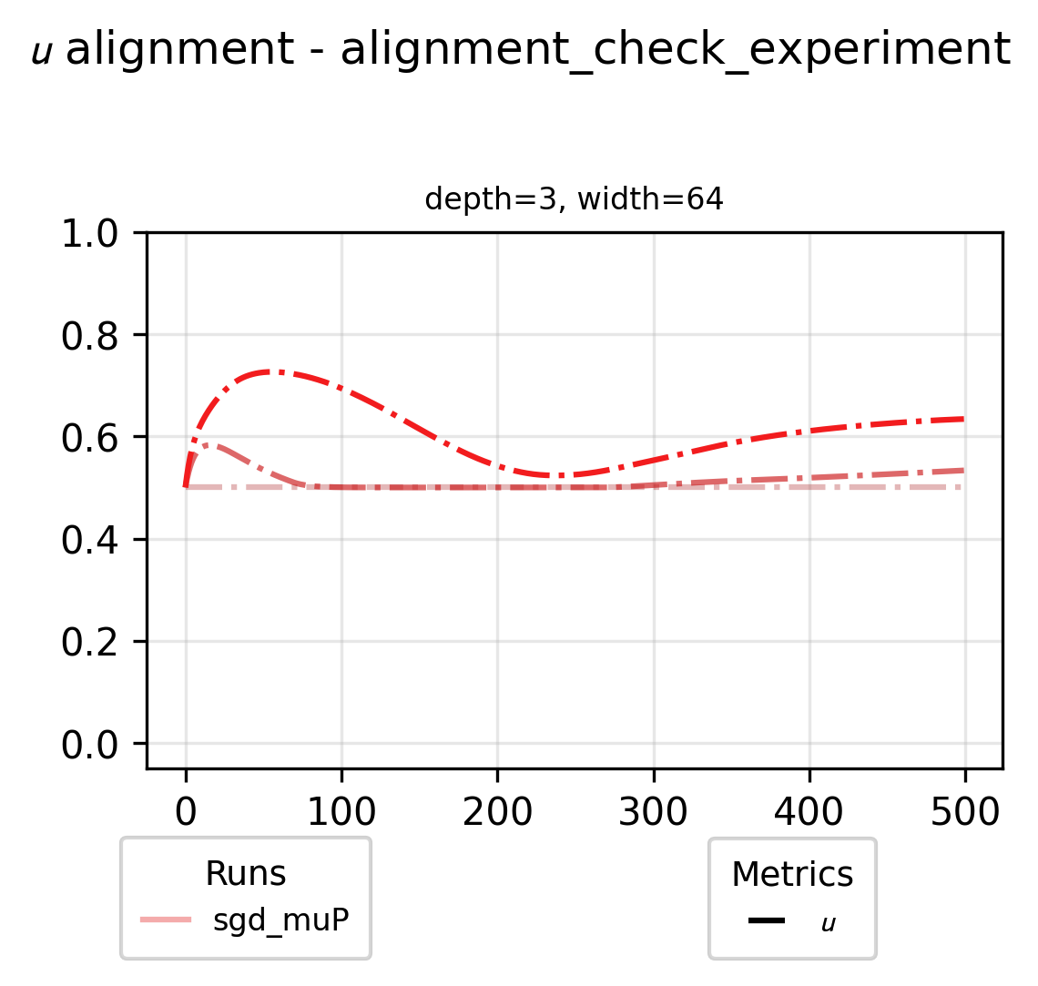
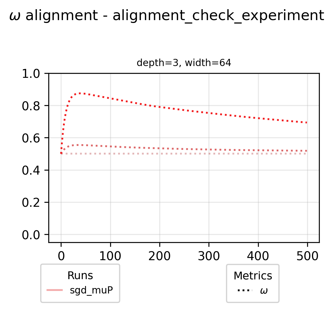
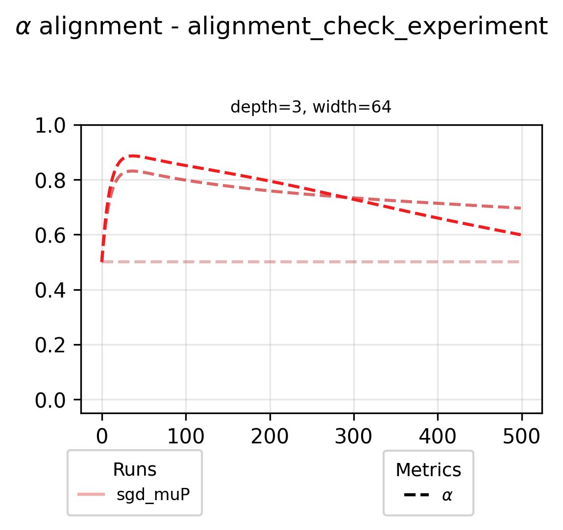
Our initial assumptions were inaccurate - full alignment would mean 0.5 omega for all layers and 1.0 U and alpha for all layers. While our omega estimates were relatively accurate, we significantly overestimated alignment for alpha and U variables. With these empirically measured alignment values, we can now update our visualization to reflect more accurate alignment assumptions.
Fascinating! By using measured alignment assumptions, we can improve our estimates of the stable training frontier!
Maximizing Update Size
Our analysis reveals a key opportunity: by overestimating alignment, we unnecessarily restrict learning rates. The full-alignment muP approach proves overly conservative. Rather than manually probing layer learning rates, we formulated this as a constrained optimization problem: maximize learning rates while satisfying our established stability inequalities. We developed a solver that accepts any ab-parameterization and alignment settings (alpha, omega, U), then outputs maximal stable learning rate exponents. By applying this to muP with our empirically measured alignment values, we discovered that for that experiment we can increase the learning rate exponent of the second layer by 0.404 (as shown in the figures). This translates to multiplying the middle layer learning rate by width^0.404 while maintaining stability. If we rerun this experiment in that setting we see the following improvement in loss:
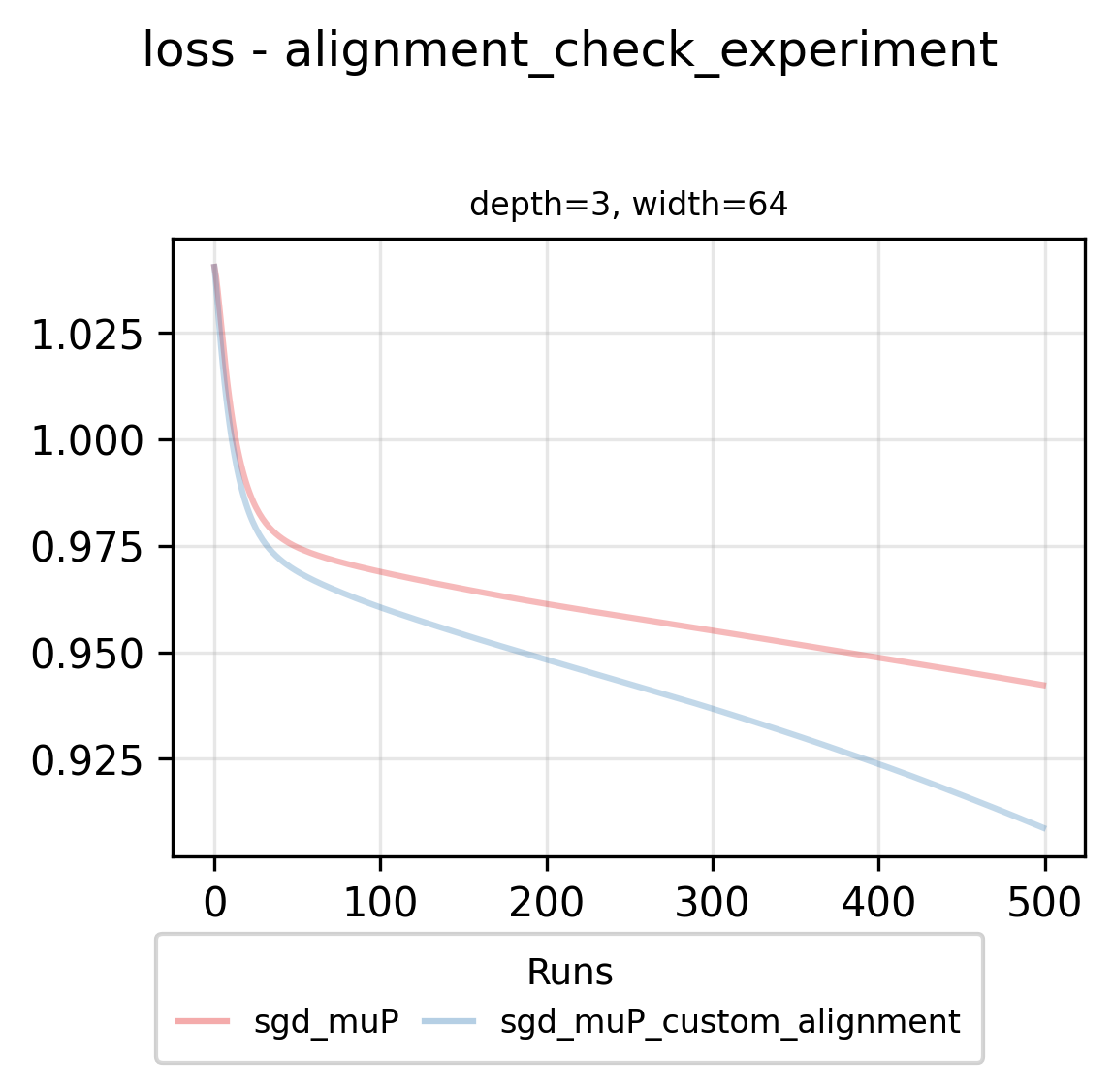
By using data-parameter alignment measurements, we minimize loss more effectively in this simple synthetic setting.
Let’s reproduce this in a slightly more challenging CIFAR-10 setting. For each experiment, we:
- Create a depth × width grid to ensure robustness across model scales
- Sweep over base learning rates and pick the best for each experiment
- Try 4 base parameterizations: mean-field, muP, standard, and NTK, all using full alignment assumptions
- Try 2 optimizers: SGD and Adam (no weight decay)
- Run each experiment for 2000 steps with batch size 256, logging loss, per-layer learning rates, alignment metrics, and activation change scale
To test our strategy:
- Start with base case using full alignment assumption and derived learning rate exponents
- Take ab-parameterization and get converged alignment variables from lowest-width version
- Derive maximal learning rate exponents using measured alignments, then run with that
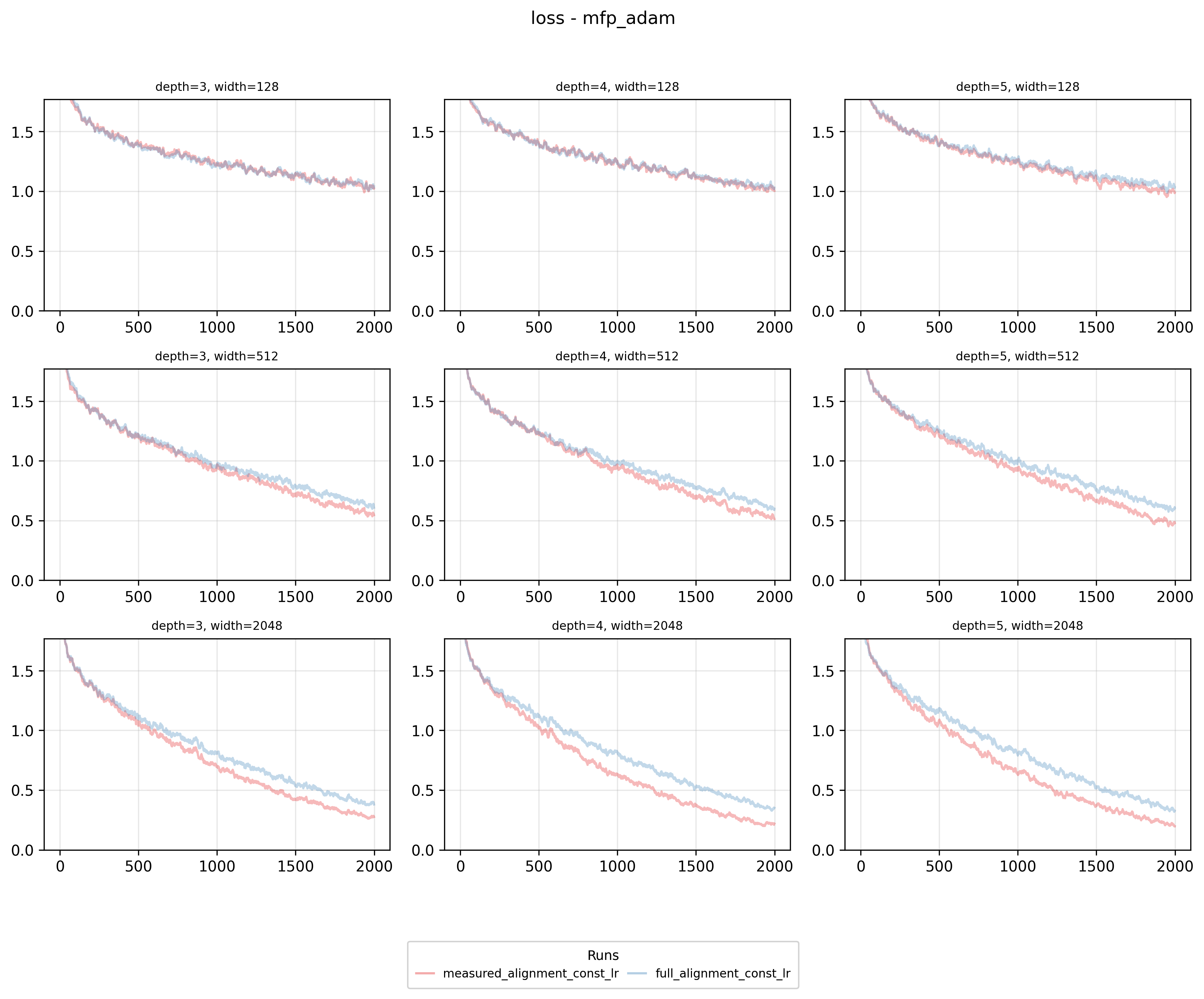
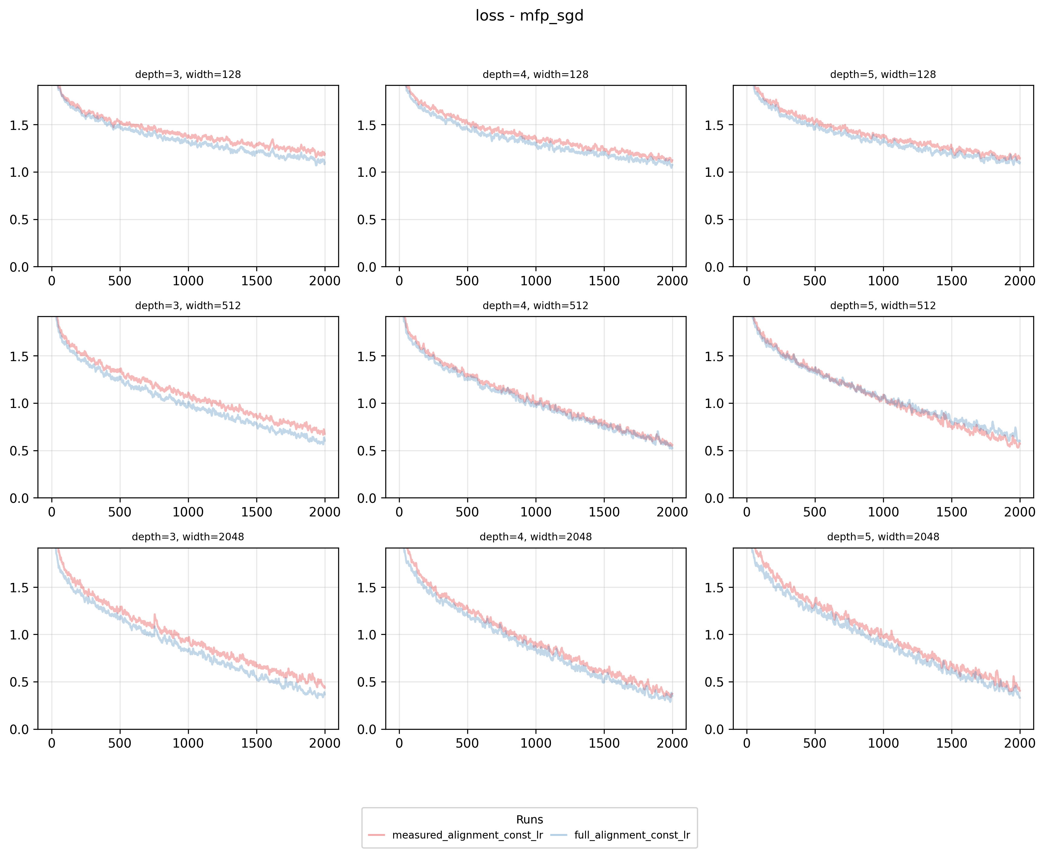
This method is practical - run a small-scale experiment to discover data-parameter alignments, then apply to your target run. For brevity, I’ll only show mean-field parameterization results, but the pattern repeats across parameterizations. Our measured-alignment-based learning rate exponents outperform full-alignment MFP for Adam, but for SGD, it’s the opposite.
Our methodology - using converged alignment variables from smaller runs to initialize larger, separate runs - rests on the assumption that alignment is primarily determined by data and parameterization choices. Since these properties remain constant across all runs in our grid, we expect the alignment patterns to generalize. To check this assumption, we can look at the absolute difference in the converged (mean across last 100 training steps) alignment variables between full alignment initialization and measured alignment initialization across different optimizers and parameterizations used in our experiments.
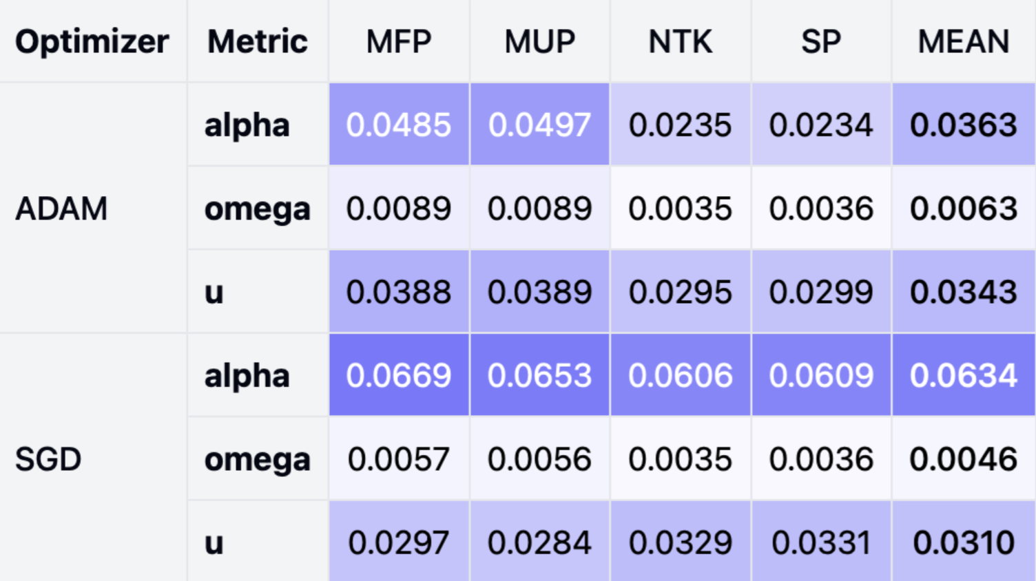
As it turns out - initial alignment assumptions influence the convergence trajectory itself, potentially invalidating our original assumptions. Consequently, our calculated “maximal” learning rate exponents may no longer be truly maximal or maintain stability. Furthermore, the results clearly show that pre-initialized alignments cause significantly greater deviation in alpha alignments with SGD compared to Adam. This suggests an important phenomenon: certain optimizers exhibit more robust alignment convergence, enabling more reliable cross-model transfer of alignment assumptions.
Dynamic Maximal LR Schedule
To address this issue, we can ensure the property of being a maximal update parameterization remains invariant throughout training. We implement this by solving for maximal learning rate exponents in real-time at each step, integrating our solver into a learning rate schedule that updates based on current alignment measurements.
select ab-parameterization: a, b
initialize weights randomly: W_init
compute initial activations: z_init = forward_pass(X, W_init)
W = W_init

for step = 1 to N:
    z = forward_pass(X)

    alpha, omega, u = compute_alignments(z_init, z, W_init, W)

    loss = compute_loss(z, y)
    gradients = backprop(loss)

    c = max_lr_solver(a, b, alpha, omega, u)
    learning_rate = update_lr_schedule(c)
    W = optimizer_step(W, gradients, learning_rate)
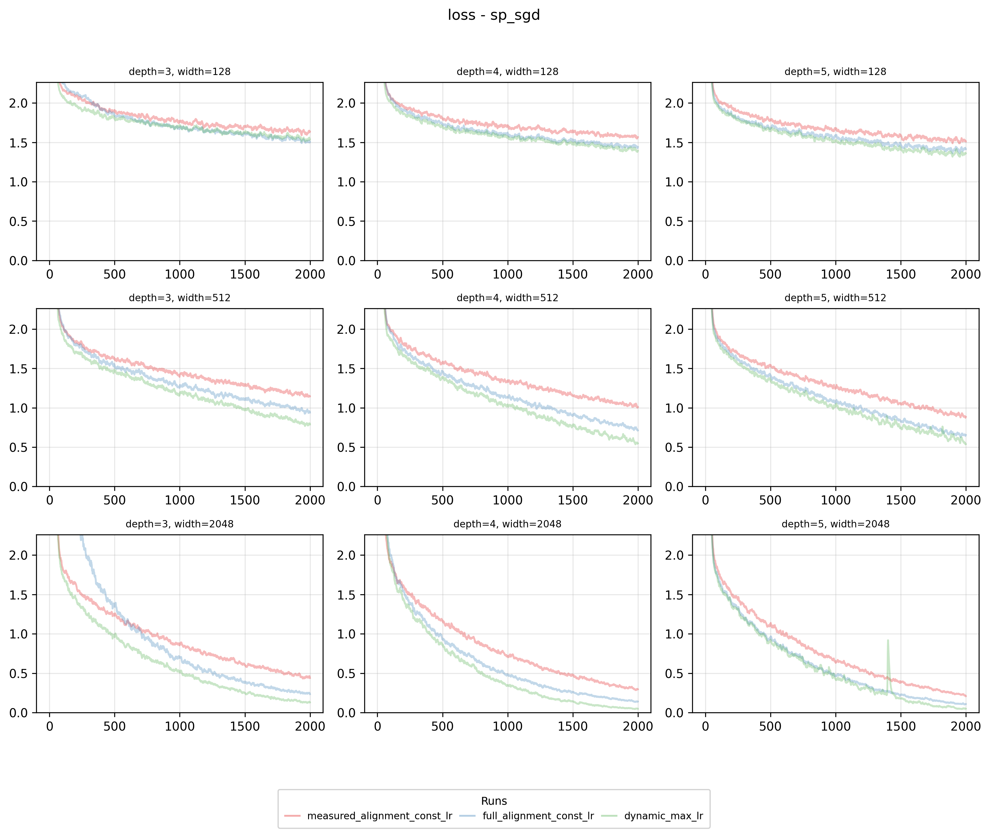
Summarizing the results: Dynamic maximal learning rate schedules consistently outperform our pre-measured method or maintain better results than baseline experiments. In the worst case, across various parameterization and optimizer combinations, we match baseline performance.
As an example of a significant improvement, here’s SP + Adam:
And here’s an example where our pre-measured alignment method underperformed but our new dynamic scheduler was able to at least match full alignment - muP + SGD:
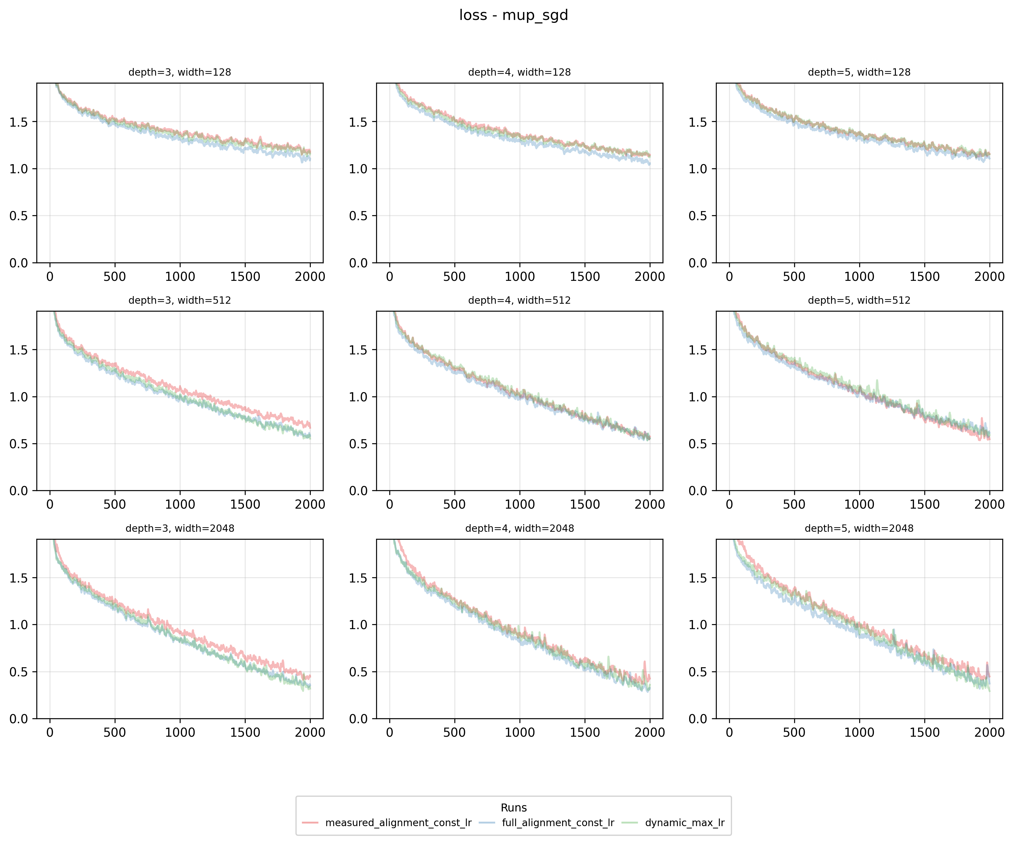
Our hypothesis for this case concerns our definition of “maximal per-layer learning rate exponents.” In our solver, we maximize the sum of learning rates, allowing tradeoffs between layers—we would reduce one layer’s rate by 0.1 if it enables increasing others by a total exceeding 0.1.
This approach assumes all layers contribute equally to optimization, which may not be universally true. If this assumption explains our inconsistent improvements, we should observe a correlation between performance and tradeoff intensity. To test this, we’ll plot loss improvement over the baseline against a metric measuring these tradeoffs - specifically, the average decrease (increases ignored) in learning rate per layer calculated as the sum of all decreases divided by the number of layers, which equals zero if all layers receive increased rates.
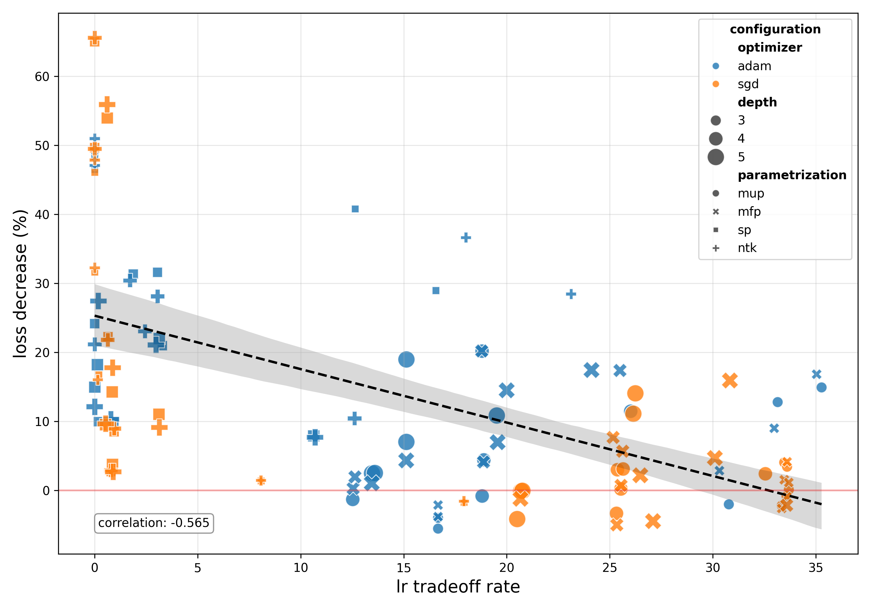
As we can see, there is a clear relationship showing that more tradeoffs lead to less loss improvement. The good thing is that in the vast majority of cases we see a healthy improvement in loss. In the future an interesting direction to look into might be a solver which only considers Pareto improvements over full alignment.
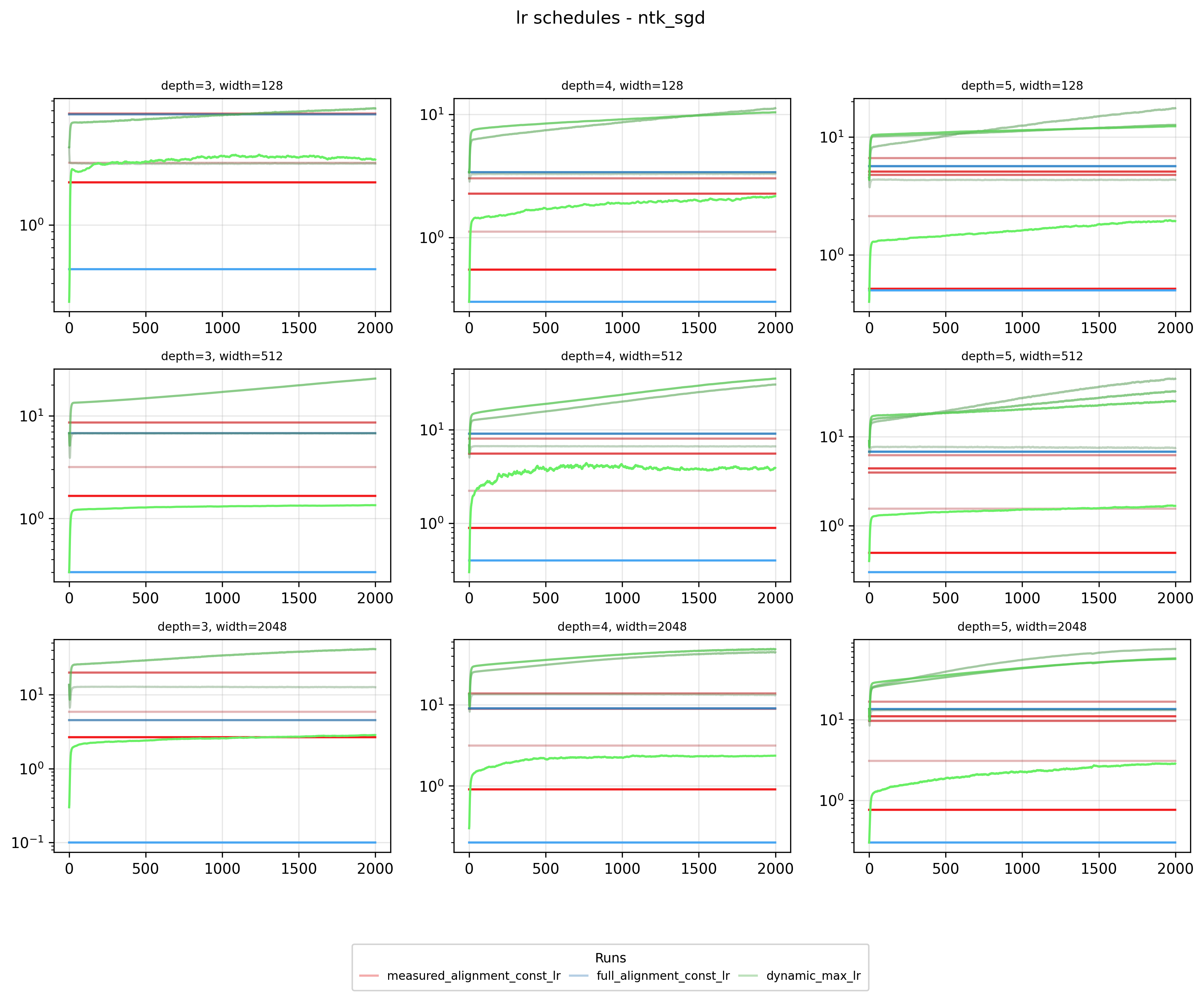
We can also see that NTK and SP parameterization dominate the lower tradeoff (left) portion of the figure whereas MFP and muP dominate the right. Furthermore in that right cluster we can see that SGD tends to have more tradeoffs than Adam. We can see what’s going on when we look at the learning rate schedule for runs from this cluster, f.e. let’s look at muP + SGD:
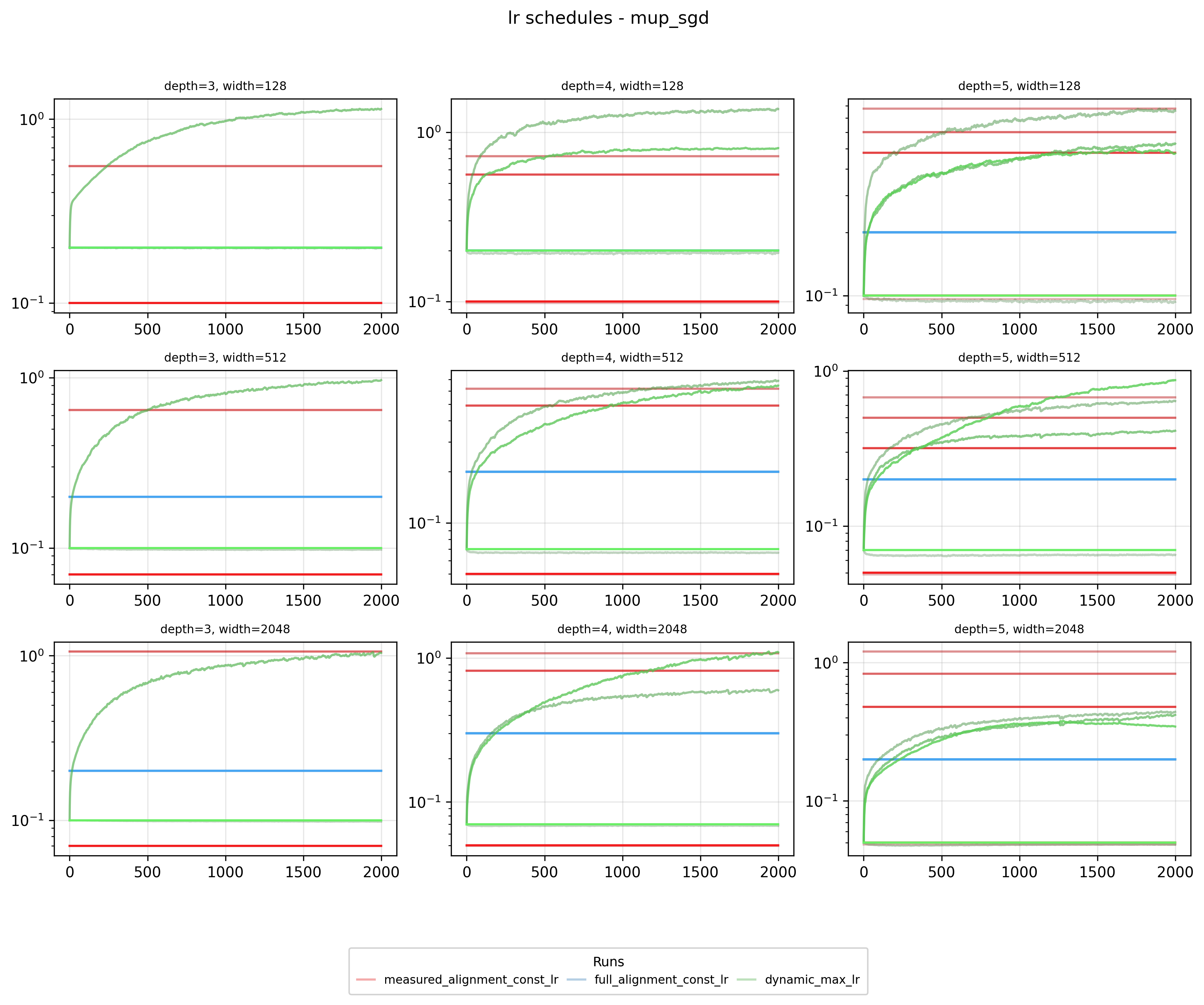
For this parameterization × optimizer, when we have full alignment, all layers get the same learning rate which means our solver will likely attempt some tradeoffs. On the other hand with NTK + SGD we can almost always get a Pareto increase in learning rate for all layers.
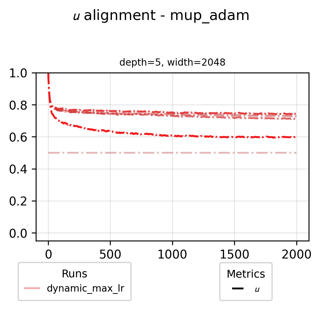
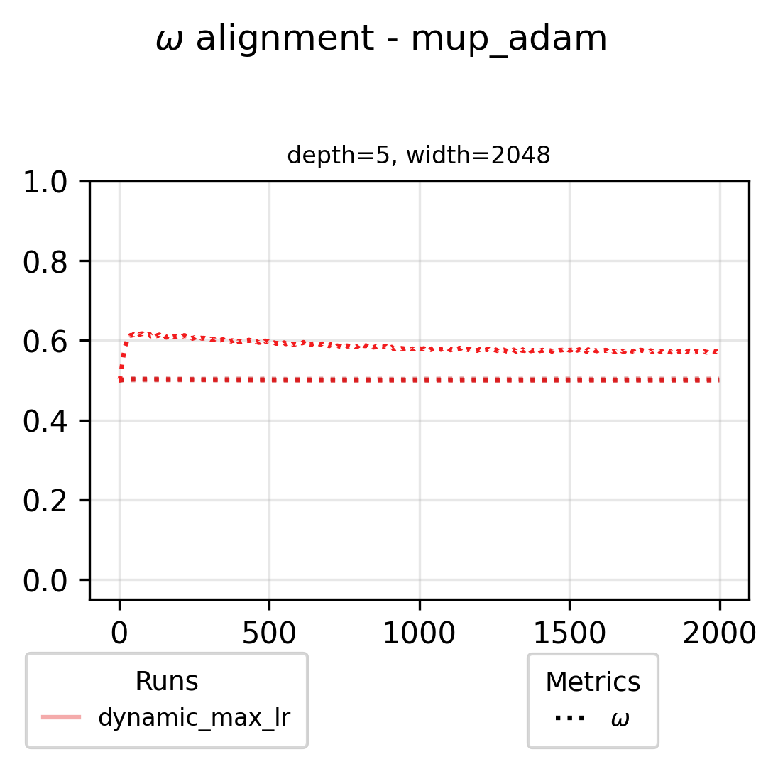
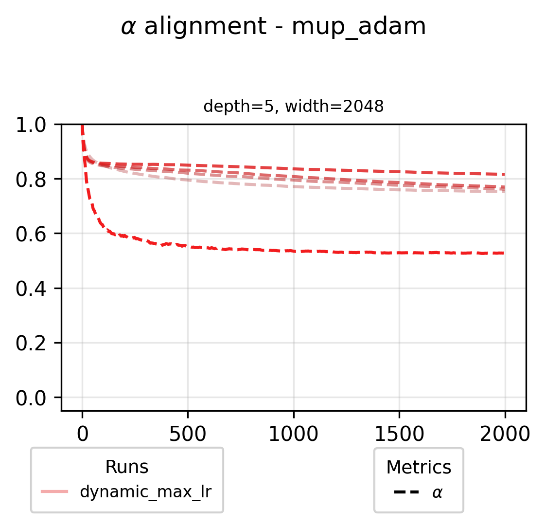
We can also check in on what the alignment variables look like for the largest scale dynamic maximal LR run in our grid (f.e. for the muP base parameterization)
What Impacts Alignment?
It’s not a unreasonable to assume that the alignment is constant and increases after training has sufficiently warmed up. To visualize this we can look at some simple math:
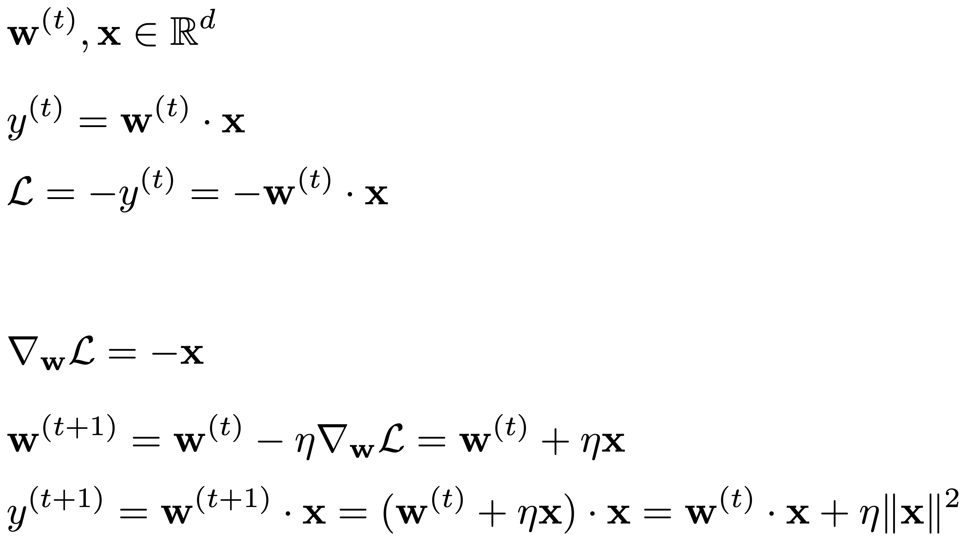
What we see above is that the primary mechanism through which the weights get updated during training is by adding “shades” of the data. Therefore it’s natural to assume the alignment would increase on the same sample. The issue with this assumption is that in most training jobs we rarely iterate over the same data and also we sometimes apply augmentations to it, like adding noise. Once again we can look at what the math in the previous example would look like if we decided to add some noise to x:
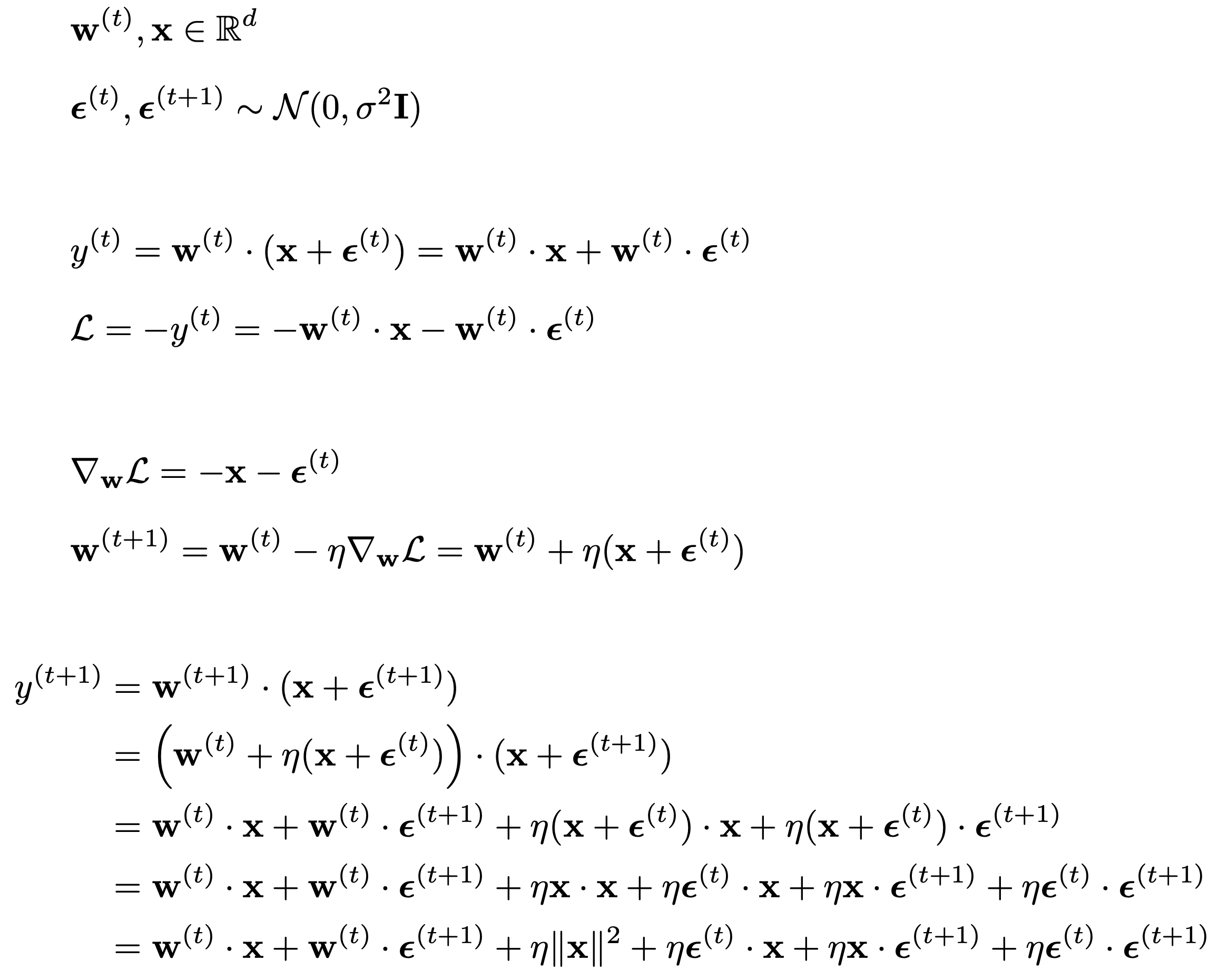
We can see that the majority of the alignment will come from the x @ x term, the rest will not be aligned. A simple example of the latter is diffusion models where at each step we will be adding noise to the data which will fundamentally limit the amount of alignment which can develop in at least the earlier layers.
To get an empirical sense of this we can pregressively add more noise to our data during training and see how the alignment variables converge. Below we can see a CIFAR-10 training run where we do a linear interpolation between the noise and the data according to the signal strength parameter:
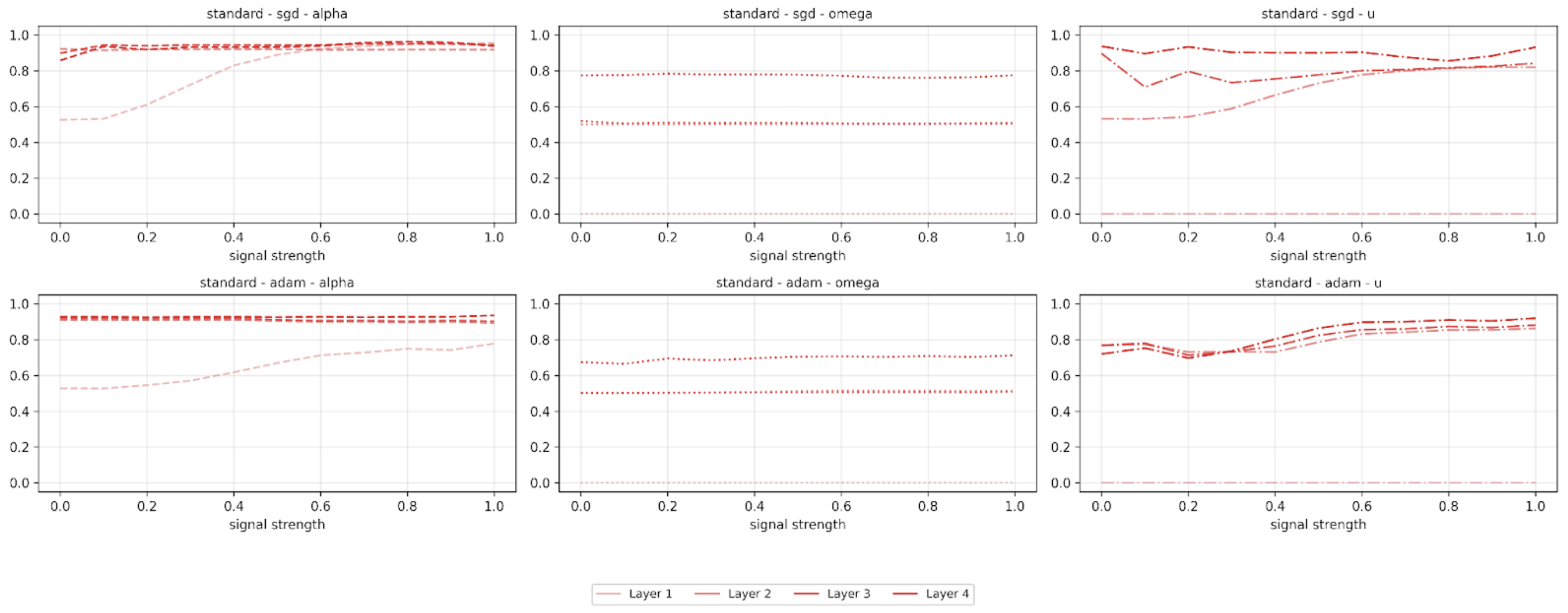
You can see that for some alignment variables, decreasing signal strength leads to decreased alignment, especially for the earlier layers.
Conclusion
Our exploration into tensor alignments confirms the findings of prior work [1] that the traditional assumption that these alignments are constant and significant isn’t always correct. In reality, they’re dynamic, and vary across network layers and training steps. We can likely unlock faster training without sacrificing stability by measuring actual alignments instead of relying on theoretical assumptions which we demonstrate for a set of simple experiments. An intriguing finding is that adding noise directly manipulates alignment properties. This suggests our approach could be especially valuable in training regimes where data characteristics change systematically such as highly multimodal or denoising-based training.
Future Work
-
Refining our “maximal” learning rate definition: Our current approach optimizes the sum of learning rates across layers, which can lead to suboptimal tradeoffs. We could explore alternative definitions that only permit Pareto improvements over full alignment or limit allowed decreases.
-
Exploring alternative alignment metrics: More suitable alignment metrics may exist. Doing this analysis with these alternative metrics could yield valuable insights.
- Investigating alignment dynamics: Several questions remain about what impacts alignment:
- Can we predict alignment decreases based on noise schedules and leverage this knowledge?
- Do multimodal models naturally exhibit lower average alignment?
- How do data characteristics influence alignment patterns?
- Developing efficient measurement techniques: To make our approach more practical, we could explore less computationally/memory intensive ways to measure alignment, such as:
- Measuring at decreasing frequency as convergence occurs
- Sharing measurements across selected subset of layers
- Estimating alignment with fewer calculations
- Integrating with existing learning rate schedules: We need to determine how our alignment-based schedules should combine with traditional schedules:
- Should we simply multiply our alignment-based schedule with standard warmup-stable-decay schedules?
- Could we replace classic linear warmup with an alignment discovery phase, after which alignment is considered constant?
- How do different combinations affect convergence properties?
References
- [1] Scaling Exponents Across Parameterizations and Optimizers (https://arxiv.org/abs/2407.05872)
- [2] The Boundary of Neural Network Trainability Is Fractal (https://arxiv.org/abs/2402.06184)
- [3] Why Momentum Really Works (https://distill.pub/2017/momentum/)
- [4] Tensor Programs V: Tuning Large Neural Networks via Zero-Shot Hyperparameter Transfer (https://arxiv.org/abs/2203.03466)
- [5] Feature Learning in Infinite-Width Neural Networks (https://arxiv.org/abs/2011.14522)
- [6] Scalable Optimization in the Modular Norm (https://arxiv.org/abs/2405.14813)
Acknowledgements
We’d like to thank Akshat Shrivastava and Armen Aghajanyan for help reviewing and editing this post as well as Katie Everett and Jeremy Bernstein for helpful discussion.
Citation
@misc{kilian2025tensoralignments,
  author       = {Maciej Kilian and Maksymilian Wojnar},
  title        = {Exploring Tensor Alignments in Neural Networks},
  year         = {2025},
  url          = {https://iejmac.github.io/2025/03/26/alignments.html}
}